Mode Connectivity

The loss landscapes of deep neural networks are highly complex and the geometric properties of them are underexplored. Mode connectivity finds that there are high accuracy pathways that connect the optima found by training independent models. The pathways between these modes can be approximated with simple curves. These paths challenge the prevailing notion of isolated local optima in high-dimensional loss landscapes.

Key Ideas

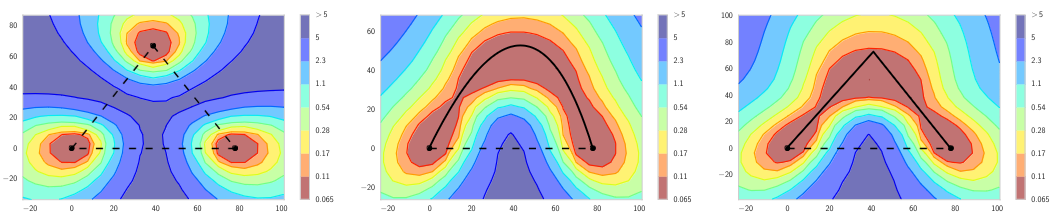
Let $\hat{w}_1$ and $\hat{w}_2$ be the weights for two independently trained networks minimized by some loss $\mathcal{L}(w)$. Let $\phi_{\theta}: [0,1] \rightarrow \mathbb{R}^{|w|}$ be a continuous piecewise smooth parametric curve with parameters $\theta$ that correspond to the network weights $\phi_{\theta}(0) = \hat{w}_1$ and $\phi_{\theta}(1) = \hat{w}_2$. The high accuracy pathway is described by the set of curve parameters $\theta$ that minimize the expectation of the loss with respect to a uniform distribution on the curve.

$$ l(\theta) = \int_0^1 \mathcal{L}(\phi_{\theta}(t))dt $$

Many parameterizations are possible with the polygonal chain and the bezier curve being used as an example in the paper. A quadratic Bezier curve provides a natural and smooth parameterization.

$$ \phi_{\theta}(t) = (1-t)^2 \hat{w}_1 + 2t(1-t)\theta + t^2 \hat{w}_2, 0 \leq t \leq 1 $$

The parameters of the curve are optimized with a standard gradient descent based approach where $\bar{t}$ is sampled from the uniform distribution $U(0, 1)$ at each itearation and steps are taken with respect to the loss $\mathcal{L}(\phi_{\theta}(\bar{t}))$.

These high accuracy pathways can be leveraged to construct low-cost ensembles via a snapshot ensemble style algorithm. Cyclic learning rate schedules are used where large learning rates encourage movement in weight space while the small rates promote convergence to accurate local minima. The learning rate schedule is a shifted annealed cosine where $\alpha_0$ is the initial learning rate, $t$ is the iteration number, $T$ is the total number of iterations, and $M$ is the number of cycles.

$$ \alpha(t) =\frac{\alpha_0}{2} \left( cos \left( \frac{\pi mod(t-1, \lceil T/M \rceil )}{\lceil T/M \rceil} \right) + 1 \right) $$

The minima found through this procedure are then used as endpoints for the curve fitting algorithm and all the weights found along the curve can be used to form independent ensemble members. This approach enables much larger ensembles of accurate members without needing to train for additional epochs.